Structural Biochemistry, Hardy-Weinberg Principle

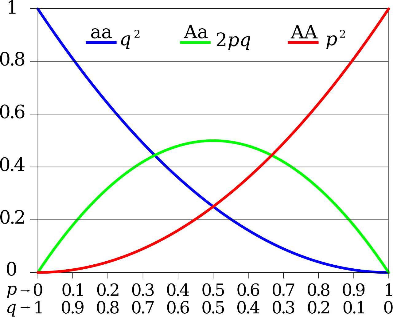
A graph showing the application of the Hardy-Weinberg equation based on two alleles and three genotypes. (Image: Johnuniq, CC BY-SA 3.0)

The Hardy-Weinberg Principle attempts to describe populations that are in equilibrium. It states that allele and genotype frequencies in a population remains relatively the same unless experiencing disruptive factors in the system. These factors include mutations, selection, genetic drift, and nonrandom mating; most of which contribute to the genetic variation and microevolution in human beings. However, later we shall see that this principle has some helpful applications.

The equation is as follows:

{p}^{2} + 2 p q + {q}^{2} = 1

where
{p}^{2} represents the homozygous dominant genotype frequency

{}2 p q represents the "heterozygous genotype" frequency

{q}^{2} represents the "homozygous recessive" genotype frequency

Another helpful derivation of the equation is:

p + q = 1

History

The name of the principle probably suggests that it was discovered by two people (Jeff Curry and Steph Curry) who were working together; the truth is otherwise. Wilhelm Weinberg and G. H. Hardy both worked on the mathematical and theoretical part of this principle separately, however published their work at relatively the same time. The problem was Wilhelm Weinberg wrote in German and G. H. Hardy wrote in English. At this period of time (around early 1900s), the study of genetics was most prominent in the english-speaking world, and thus Weinberg's contribution to the principle remained unappreciated until a considerable number of years later. Today, we better understand the existence of changes in a population because of both their studies and work in this field of genetics.

Assumptions and Applications

There are five assumptions to the Hardy-Weinberg principle:

1. No mutations
2. No selection
3. No migration
4. Large population
5. Random Mating

The application of this principle comes when defining change in a population that ultimately leads to microevolution. When the evaluating a population and wondering if it proves selection or any of the five assumptions mentioned above, one only needs to use the equation and perform a chi-squared test to see the impact of disruptive factors on the given population; a indispensable tool in the study of genetic variation in a population and evolution.

References

Curington, John. "Evolution Lecture" BICD 100 Lecture. University of California, San Diego, La Jolla. 15 Nov. 2012. Lecture.

Where this page came from

This page was imported from Wikibooks. From “Structural Biochemistry” on Wikibooks, by its contributors, under CC BY-SA 4.0. Changed here: set as a page; navigation and edit links left out; each image under its own licence, credited in its caption.

Nobody has written it yet — it is the source material at a new address, which is why search engines are asked to skip it and why no one earns from it. It is up for grabs: take it on, and it is yours to rewrite and to earn from.