The magnetic charts of the United States for Epoch 1975

GEOLOGICAL SURVEY CIRCULAR 81 0

GEOLOGICAL SURVEY CIRCULAR United States Department of. the Interior

Conclusion....................................................................

By E. B. Fabiano, W. J. Jones, and N. W. Peddie within the COT48 region and 8,036 locations in Alaska. considered acceptable only if both H and Z were measured at the station. Some 70 percent of the data were measured prior to 1963, and more than one-half of the entire file were obtained from the airborne surveys conducted by the u.s. Naval Oceanographic Office and the Department of Energy, Mines and Resources of Canada. Airborne survey data now constitute more than 85 percent of the survey file measured since 1953.

The file of measurements obtained from 1900 to 1962 had been previously reduced for the 1965 series of magnetic charts. the reduction procedure for this subset of data involved correct ions for the last few years of the previous update (1962.5-1965.0) and the application of the more recent secular variation until the epoch date of 1975.0. data were corrected to sea level using an approximation suggested by Chapman (1951). small heights (h) measured in kilometers, any component will be decreased by a fraction h/2123 of itself at height h.

To identify and remove what appear to be erroneous or anomalous values, residuals were computed for each measurement using the world magnetic charts model for epoch 1970 (Hurwitz and others, 1974) as the reference field and 1967.5 as the reference date. residuals exceeding 800 nT (1,000 nT for Alaska) were rejected and, as a result of this screening process, 12 percent of the original file was omitted from the analysis.

Appendix A shows the distribution of H and Z observations used in obtaining the tessera means for the COT48 region. The gaps represent the areas where no H and Z measurements were available. area lacked vector data, values were synthesized from AWC75 and used to supplement this file for each 2° by 2° gap.

Because relatively few D measurements had been acquired since the last series of D charts, published in 1970, the decision was made to synthesize one value for each one-degree quad from these charts, apply SV (secular variation) corrections from 1967.5-1975.0 and then perform the least-squares analysis.

The file used for the SV analysis consisted of three categories of data:

1. The annual mean values of D, H, and Z from Canadian and u.s. magnetic observatories.
2. Vector field measurements at some 100 repeat stations in COT48, which are occupied every 5-7 years.
3. Supplemental values of annual change, synthesized from AWC75. These consisted of values on a 3° x 3° grid in the ocean

A record for each location was

For Alaska, since one-third of the

Secular Variation Data Consequently,

Data with no repeat station data since 1965 were available on time to perform a regional SV analysis for Alaska. annual change from AWC75 were used to derive the SV polynomial coefficients. the Alaskan repeat stations which, nevertheless, were useful in the subsequent evaluation.)

1967.5-1975.0, the linear rates of change for D, H, and Z were determined by straight lines fitted to the OAM (observatory annual means) and the repeat-station measurements. reviewed for errors, and on the basis of a preliminary analysis, the observatory rates were given seven times greater weight than the repeat-station rates.

procedure is of the form

where K is the linear rate of change; n, the degree of the polynomial; a 11 , the coefficients to be determined; and 9c' -xc' the normalized geographic coordinates. were nor~lized so that ec = e - 52° and Ac = A - 268 • Here, 9 longitude.

(15 and 28 coefficients respectively). basis of the rms deviations, shown in table 1, the latter models were adopted for final use.

means for each one-degree tessera, and the data were functions of the form described in the section entitled "SV Analysis for COT48." run for n=4, 7, and 9, with the objective of determining the optimum fit with the fewest number of coefficients. Finally, the models for n=7 were adopted. For Alaska, the analysis presented two difficulties:

1. The data-selection region for Alaska,

areas and were included to minimize edge effects at the chart borders.

At the time this chart was being compiled,

Therefore, for Alaska, grid values of

The function adopted for the least-squares

Analyses were performed for degrees 4 and 6

Values of H and Z were averaged to obtain

subsequently analyzed using polynomial

consisting of 2,556 one-degree SV Analysis for COT48

Main Field Analysis (Appendix B lists

colatitude and A = east

s.s

s. 8

z

Table 5 refers to the partitioning scheme and related statistics for the D models of COT48. Because the values analyzed are scaled from a smooth chart, the overall fit, as one might anticipate, is remarkably close, to within 6 minutes of arc for most partitions, providing some evidence for the adequacy of the modeling process for regions as large as 2 million square kilometers--the partitioned area. bands 2 and 3 probably indicate the numerous declination anomalies in the Great Lakes region.

The D models were also evaluated by comparing them to two subsets of survey data. The first set consisted of 1,450 station values, updated to 1975.0 and randomly distributed within COT48. overall rms of 0. 50° was determined. The second subset, comprising survey data excluded from the file of analysis data, consisted of 287 airborne measurements from the Project Magnet surveys made from 196 7 to 1970. computed rms was 0.52°.

Among the reasons for the lack of fit that one may observe from the differences which exist between the data and models, the following should be noted:

1. Errors in the data. This problem was discussed earlier. Wherever possible, it is important to determine whether the errors are random or systematic. Hannaford and Haines (1969), for example, reported probable errors in aeromagnetic data of 0.4° in D, 40 nT in H, and 70 nT in z. In the older land survey data, Deel and Howe (1948) reported possible errors as large as 150 nT in the computed value of Z due to instrumental uncertainties.
2. Secular variation. The secularvariation estimates for the earlier years, especially prior to the 1930's, are less reliable, due primarily to insufficient data as well as to the quality of the instrumentation. In addition, the use of linear SV estimates, though

approximate size of each The larger rms values in

From these measurements, an

With this set, the convenient and in some instances practical, introduces errors in data reduction because the SV is not necessarily linear. This is not a serious problem for datareduction intervals of a few years. However, for a 5- or 10- year interval, significant errors could accumulate.

3. Local and regional anomalies. It is difficult at this time to assess the impact resulting from the local and regional magnetic anomalies on the statistics relating to the fit of the data to the model. If, for example, one had available up-todate vector measurements spaced a few kilometers apart nationwide, relatively accurate assessments of the "normal" and anomalous fields could be made. To date, however, the available vector data are too poorly distributed, both in space and in time.

A small-scale chart of total intensity and its annual change for 1975 in the United States is shown in figure 1. the 1975 U.S. total intensity chart (Fabiano and others, 1976). estimates of total intensity (FOOT) can change over a 10-year period. 45° and longitude 90° the estimated rates of SV differ by more than 60 nT/yr.

The various statistics of fit presented indicate that generally adequate for producing models of the smoothed field suitable for national reference charts. The major deterrent for obtaining mre reliable models appears to lie not so much in technique as it does in the accuracy of the available data base.

Dependence on these data may soon be minimized and perhaps eliminated as a result of two magnetic surveys, one completed and the other planned. Oceanographic Office completed a vector survey of the United States with north-south tracklines flown at approximately lOQ-km spacing; several east-west lines were also flown. National Aeronautics and Space Administration in cooperation with the U.S. Geological Survey will launch MAGSAT, a low-level satellite which will obtain worldwide vector data. of measurements substantially improve the data base used for future national charts.

This chart was adapted from

Figure 2 illustrates how SV

Note that at latitude

During 1977-78, the u.s. Naval

from both technique is

The acquisition sources will

.Jo·--------

.Jo.

L

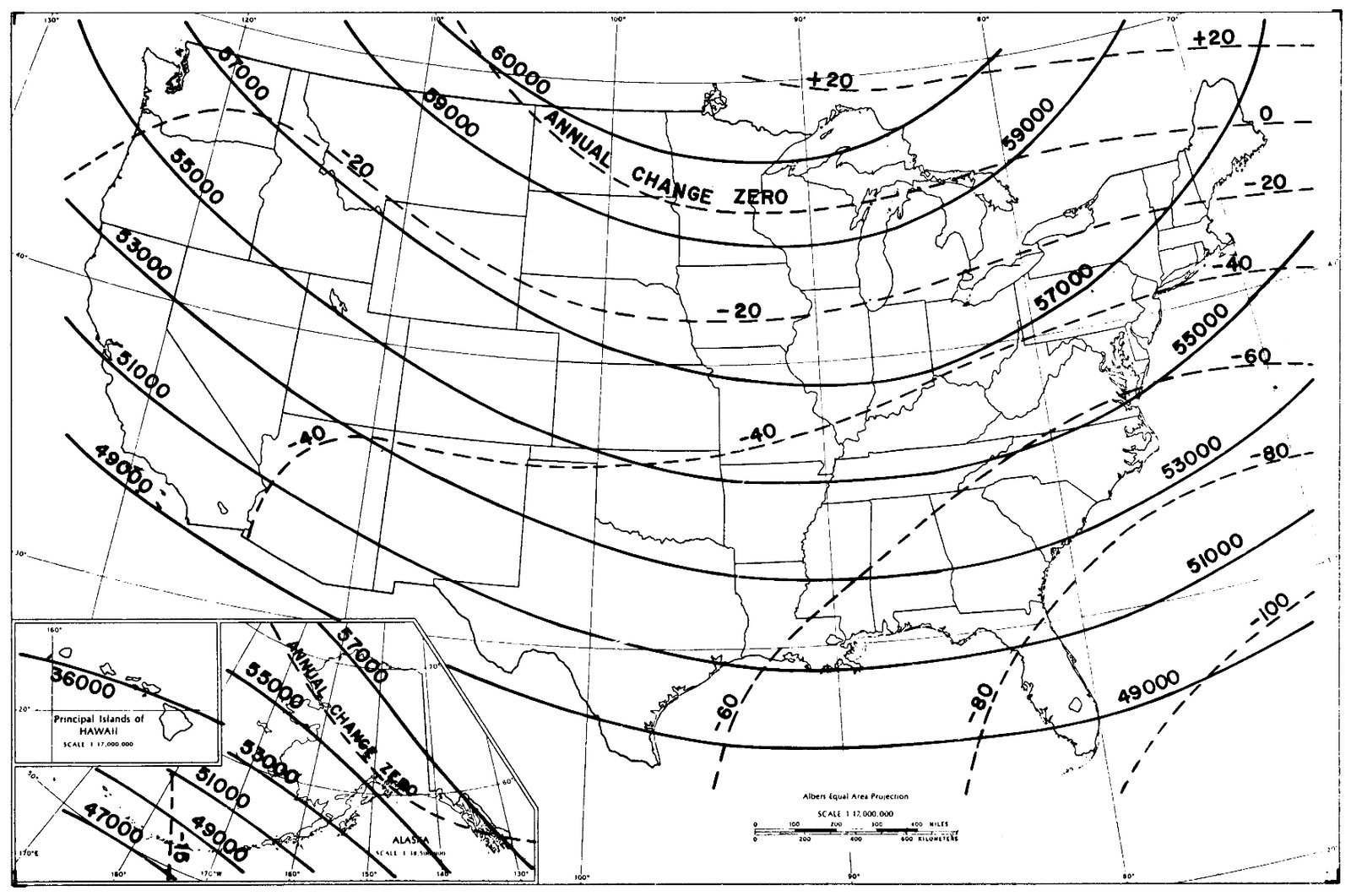
Figure 1. Total Intensity in the United States for 1975. (Solid lines are field contours in units of nanotesla (nT); dashed lines are annual change contours in units of nT/yr.)

[Station value minus model value for the date of measurement; for example, 19 71. 4 = 71. 4; Lat, latitude; Long, longitude; Decl, declination; Horiz, horizontal; Vert, vertical;

AL--- AL---- AL---- AZ---- AZ----

CA---- CA---- CA---- CA---- CA----

co----

FL---- FL---- FL---- FL---- FL----

GA---- GA---- GA---- GA---- ID----

IL---- IL---- IA---- KY---- ME----

ME---- ME---- ME---- MI---- MI----

MI---- MO---- MS---- MS---- MS----

MS---- MT---- MT---- MT---- MT----- degrees; nT, nanotesla]

Station (name)

Marion (FISH)--------- Marion (FISH)--------- Gadsden--------------- Nogales--------------- Phoenix---------------

Bishop---------------- Lompoc---------------- San Diego (CAMP ELL2)- San Diego (MIRAMAR)--- San Francisco (1952)--

San Francisco (GOLF)-- Cortez (ARPT)--------- Fort Meyers----------- Fort Meyers----------- Key West (RK PT)------

Key West (GOLF)------- Key West (GOLF) Aux-2- Spruce Creek (TEL)---- Spruce Creek (A)------ Spruce Creek----------

Bainbridge (1958) ----- Bainbridge (1958)----- Milledgeville--------- Waycross-------------- Weiser----------------

Joliet (CC 2)--------- Joliet (WDRF) --------- Indianapolis---------- Lexington (CC)-------- Bangor (BROADWAY)-----

Bangor (GRIFFIN)------ Fort Kent (B HOSP)---- Fort Kent (PASTURE)--- Detroit (PARK)-------- Detroit (RR)----------

Marquette (GF2 197 2)-- Rolla (EAST)---------- Brooklyn-------------- Grenada (A)----------- Granada (71)----------

Lamar (B GUM)--------- Billings (PP)--------- Glendive (ARPT 71)---- Havre----------------- Helena (ARPT 71)------ Lat

30.92 45.79 47.13 48.56 46.60 Long

-89.39 -108.53 -104.81 -109.72 -111.98 Decl

0.06 -0.72 -0.17 0.02 -0.36 Dip

o. 01

o.oo

o.oo

o.oo

o.oo

0.10 -0.07 Horiz nT

122. -246. Total nT

72.9 72.5 71.6 71.5 71.6 Appendix B.--Residuals--u.s. reeeat stations and observatories 1 including Alaskan reeeat stations

MT---- MT---- MO---- MO---- NE----

NE---- NE---- NE---- NV---- NV----

NV---- NH---- NH---- NM---- NM----

NM---- NM---- NY---- NY---- NC----

NC---- NC---- NC---- ND---- ND----

ND---- NO---- OK---- OK---- OR----

OR---- PA---- PA---- RI---- RI----

sc---- SD---- SD---- TN---- TX----

TX---- TX---- TX---- TX---- TX----

TX---- TX---- TX---- UT---- --Continued.

Station (name)

Helena (GR MDW)------- Helena (ARPT 2)------- Carrollton------------ Rolla (WEST)---------- Fremont (ARPT-64)-----

Fremont (ARPT-7 3) ----- Halsey (B 73)--------- Fremont (ARPT)-------- Ely (BLM)------------- Las Vegas (M GLF)-----

Winnemuca (ARPT)------ Keene (ARPT)---------- Surry----------------- Deming---------------- Deming (ARPT 72)------

Hobbs----------------- Soccoro (ARPT 72)----- Syracuse (DRUM)------- Syracuse (DRUM B)----- Wadesboro-------------

Wilmington (GOLF 1)--- Wilmington (GOLF 2)--- Wilmington (GOLF 2)--- Bowbells-------------- Jamestown-------------

Jamestown (ARPT)------ Pembina (PARK)-------- Carmen (PARK)--------- Tulsa (LEONARD)------- Burns (FGNDS)---------

Eugene (RESV)--------- Indiantown Gap (AF)--- Indiantown Gap (LAKE)- Kingston (CAMPUS)----- Kingston (TURF)-------

Fort Jackson---------- Belle Fourche 2------- Huron (CC)------------ Clarksville 73-------- Brownsville (GOLF 2)--

Austin (DS)----------- Austin (GOLF)--------- Hereford-------------- Laredo (NORTH)-------- Laredo (WEST)---------

Orange (C)------------ Van Horn (1972)------- Pandale--------------- Cedar City (ARPT)----- Lat

30.06 31.05 30.21 37.70 Long

-93.80 -104.84 -101.37 -113.09 Decl

-0.74 -0.50 -0.20 -0.64 o.ss -0.03

o.os

0.08 o.oo -0.11 -0.32 -0.19 Dip

0.18 o.os -128. -144. -187. 72.9 0.04 0.03 0.67

-0.26 0.16 Horiz nT

72.9 72.8 72.8 73.8 Appendix B.--Residuals.--u.s. re:2eat stations and observatories 1 including Alaskan re:2eat stations

UT---- VT---- VT---- WA---- WA----

WA---- WA---- WI---- WI----

co----

CA---- TX---- AZ---- AK---- AK----

AK---- AK---- AK---- AK---- AK----

AK---- AK---- AK---- AK---- AK----

AK---- AK---- AK---- AK---- Ak----

AK---- AK---- AK---- AK---- AK----

AK---- AK---- AK---- AK---- --Continued.

Station (name)

Salt Lake City-------- Burlington (LP) ------- Burlington (RS)------- Coulee Dam------------ Quillayute------------

Newport Boulder -------------- Fredericksburg

Castle Rock Dallas Tucson Anchorage (NBS)------- Barter Is (IGY)-------

Bethel (AIRPORT)------ Chitina--------------- Cordova 3 (1975) ------ Fort Yukon (IGY)------ Homer 1 (AIRPORT)-----

Nome (APT) Aux A (58)- Northway (IGY) 2------ Platinum-------------- Pt Hope (CEMETERY)---- Prudhoe Bay (1975) ----

Ruby 3 (1975)--------- Seward---------------- Shungnak-------------- Unalakleet (1975) ----- Unalaska--------------

Yakutai 5 (1975)------ Barrow --------------- Collete -------------- Sitka ----------------

Observatory.

---------- --------------- --------------- Lat

59.51 71.30 64.86 57.06 Long

-139.66 -156.75 -147.84 -135.33 Decl

0.19 0.21 -0.67 o. 71 -0.12 0.46

-0.21 0.46 0.26 0.13 Dip

o.oo

0.16 -0.07 0.06 -0.08 Horiz nT

63. Vert Total nT

Where this page came from

This page was imported from U.S. Geological Survey. Published by the U.S. Geological Survey and, as a work of the United States government, in the public domain.

Nobody has written it yet — it is the source material at a new address, which is why search engines are asked to skip it and why no one earns from it. It is up for grabs: take it on, and it is yours to rewrite and to earn from.